Milestone: CMEPS 0.3
- Overview
- Supported Compsets
- Supported Platforms
- Limitations and Known Bugs
- Download, Build, and Run
- Frequently Asked Questions
- Validation
- Appendix with additional plots
This milestone is a release of the Community Mediator for Earth Prediction Systems (CMEPS) with the ability to reproduce the behavior of the existing Mediator in the NOAA Environmental Modeling System (NEMS) used in the Unified Forecast System (UFS). The release includes a test configuration (compset) of the UFS Subseasonal-to-Seasonal coupled application consisting of the Finite Volume Cubed Sphere - Global Forecast System (FV3GFS) atmospheric model, the Modular Ocean Model (MOM6) and the Los Alamos Sea Ice Model (CICE5). The workflow is provided by the Common Infrastructure for Modeling the Earth (CIME).
The purpose of this milestone is to demonstrate that the CMEPS Mediator is capable of reproducing the same behavior as the existing NEMS Mediator in the context of the UFS Subseasonal-to-Seasonal application and is poised to replace the NEMS Mediator. This milestone is validated by running the same configuration as the UFS Subseasonal-to-Seasonal coupled system but using the CMEPS Mediator in place of the NEMS Mediator.
CMEPS and CIME were extended to support existing behaviors used in the UFS Subseasonal-to-Seasonal system to reduce any differences between the systems. UFS uses a special sequential cold start run sequence to generate an initial set of surface fluxes. The system is then restarted with only the Mediator reading in the initial fluxes and the atmosphere, ocean, and ice components reading in their initial conditions. This behavior is reproduced using CMEPS. See the FAQ for specific instructions on how to generate an initial set of surface fluxes and restart only the Mediator.
The NEMS Mediator is not currently fully conservative when remapping surface fluxes between model grids: a special nearest neighbor fill is used along the coastline to ensure physically realistic values are available in cells where masking mismatches would otherwise leave unmapped values. Although CMEPS has a conservative option and support for fractional surface types, the NEMS nearest neighbor fills were implemented in CMEPS so that the two Mediators would have similar behavior. In a future release, the fully conservative option will be enabled.
Four 35-day CMEPS runs were compared against a set of recent benchmarks conducted with UFS, focusing on ice concentration, thickness, and total area; sea surface temperature; and surface heat flux components. The results indicate that the large scale spatial distribution and time evolution of the ice are generally reproduced, although there are differences in total ice area in the southern hemisphere and some differences in finer spatial distribution along the coastlines. Sea surface temperatures (SSTs) are consistent between the systems and average SST shows strong correlations especially up to day 10 of the simulation for all subregions analyzed. There is no spatial systematic bias indicated in SST. There are inconsistencies in the net shortwave radiation received by MOM6, especially at the first 6 hour output. Differences in shortwave, longwave, latent heat, and sensible heat fluxes grow as the system evolves in time. This requires further investigation.
A compset is a specific configuration of components in a coupled system including a set of grid resolutions. The following compset is supported in this milestone.
- UFS_S2S (FVGFS-MOM6-CICE5): Fully active configuration of coupled atmosphere, ocean and ice components. Supported resolutions:
- C384_t025 (atmosphere: C384 cubed sphere, ocean/ice: 1/4 degree tripolar)
- Theia/NOAA - 35 day runs for four initial conditions (January, April, July, October 2012) were performed on this platform.
- Cheyenne/NCAR - a set of 5 day and shorter runs were performed on this platform.
- Stampede2/XSEDE - a set of 5 day and shorter runs were performed on this platform.
This milestone release has the following limitations:
-
There are several known differences between the NEMS benchmark runs and the CMEPS runs used for the validation:
- The codebases used for MOM6 and the MOM6 NUOPC caps differ. There is a unified MOM6 codebase/cap that will be used for future runs. This unified cap includes bug fixes that affect model output.
- The codebases used for the CICE model and NUOPC cap differ. Both systems are using a version of CICE5, but the codebases are not identical. Every effort was made to make the ice namelist parameters as close as possible between the two systems. A formal analysis of the code differences has not been completed.
- The NEMS benchmark runs were run with ESMF 8 beta snapshot 1 (8bs1) and the CMEPS runs used ESMF 8 beta snapshot 29 (8bs29). The latter snapshot includes a fix to improve calculation of cell areas over 90 degrees. This affects results in the regridding of fields between components.
-
The FV3GFS repository is not publicly available so a local git repository is provided on each supported platform.
-
MOM6 and FV3 must be run on separate sets of processors due to an interaction with FMS when both are called on the same processors. This is the default configuration and is preferable anyway because it allows for concurrency in the system.
# Clone UFSCOMP umbrella repository
$ git clone https://github.com/ESCOMP/UFSCOMP.git
$ cd UFSCOMP
# To checkout the tag for this milestone:
$ git checkout cmeps_v0.3
# To checkout the development branches (with continued commits):
$ git checkout app_fv3gfs-cmeps

# Check out all model components and CIME
# IMPORTANT: Use the appropriate Externals files for your platform

# Cheyenne:
$ ./manage_externals/checkout_externals

# Stampede2:
$ ./manage_externals/checkout_externals -e Externals.Stampede2.cfg

# Theia:
$ ./manage_externals/checkout_externals -e Externals.Theia.cfg

# Create UFS S2S case using the name "ufs.s2s.c384_t025" (the user can choose any name)
$ cd cime/scripts
$ ./create_newcase --compset UFS_S2S --res C384_t025 --case ufs.s2s.c384_t025 --driver nuopc --run-unsupported

# Setup and Build
$ cd ufs.s2s.c384_t025  # this is your "case root" directory selected above, and can be whatever name you choose
$ ./case.setup
$ ./case.build

# Turn off short term archiving
$ ./xmlchange DOUT_S=FALSE

# Submit a 1 hour cold start run to generate mediator restart
$ ./xmlchange STOP_OPTION=nhours
$ ./xmlchange STOP_N=1
$ ./case.submit

# Output appears in the case run directory:
# On Cheyenne:
$ cd /glade/scratch/<user>/ufs.s2s.c384_t025

# On Stampede2:
$ cd $SCRATCH/ufs.s2s.c384_t025

# On Theia:
$ cd /scratch4/NCEPDEV/nems/noscrub/<user>/cimecases/ufs.s2s.c384_t025
The --res flag is used to create a case with different horizontal resolution. For example, the following commands modify the horizontal resolution for each model components in the UFS_S2S compset:
# FV3 is in C96 (1.0 degree) and MOM (and CICE) is in 0.25 degree resolution
./create_newcase --compset UFS_S2S --res C96_t025 --case ufs.s2s.c96_t025 --driver nuopc --run-unsupported
# FV3 is in C384 (0.25 degree) and MOM (and CICE) is in 0.25 degree resolution
./create_newcase --compset UFS_S2S --res C384_t025 --case ufs.s2s.c384_t025 --driver nuopc --run-unsupported
The PE layout affects the overall performance of the system. The following command shows the default PE layout of the case:
cd /path/to/UFSCOMP/cime/scripts/ufs.s2s.c384_t025
./pelayout
To change the PE layout temporarily, the xmlchange command is used. For example, the following commands are used to assign a custom PE layout for the c384_t025 resolution case:
cd /path/to/UFSCOMP/cime/scripts/ufs.s2s.c384_t025
./xmlchange NTASKS_CPL=312
./xmlchange NTASKS_ATM=312
./xmlchange NTASKS_OCN=360
./xmlchange NTASKS_ICE=24
./xmlchange ROOTPE_OCN=312
./xmlchange ROOTPE_ICE=672
This will assign 312 cores to ATM and CPL (Mediator), 360 cores to OCN and 24 cores to ICE components. In this setup, all the model components run concurrently and PEs will be distributed as 0-311 for ATM and CPL, 312-671 for OCN and 672-696 for ICE components.
To change the default PE layout permanently for a specific case:
# Goto main configuration file used to define PE layout
cd /path/to/UFSCOMP/components/fv3/cime_config/config_pes.xml
# And find specific case and edit ntasks and rootpe elements in the XML file.
# For example, a%C384.+oi%tx0.25v1 is used to modify default PE layout for c384_t025 case.
For a new case, pass the --walltime parameter to create_newcase. For example, to default the job time to 20 minutes, you would use this command:
$ ./create_newcase --compset UFS_S2S --res C384_t025 --case ufs.s2s.c384_t025.tw --driver nuopc --run-unsupported --walltime=00:20:00
For an existing case, you can change the job walltime time using xmlchange inside the case directory:
$ ./xmlchange JOB_WALLCLOCK_TIME=00:20:00
The coupled system should be run for at least 1 day forecast period before restarting. To restart the model, re-submit a case after the previous run by setting CONTINUE_RUN XML option to TRUE using xmlchange.
$ cd /path/to/UFSCOMP/cime/scripts/ufs.s2s.c384_t025  # back to your case root
$ ./xmlchange CONTINUE_RUN=TRUE
$ ./xmlchange STOP_OPTION=ndays
$ ./xmlchange STOP_N=1
$ ./case.submit
In this case, the modeling system will use the warm start run sequence which allows concurrency.
To run the system concurrently, an initial set of surface fluxes must be available to the Mediator. This capability was implemented to match the existing protocol used in the UFS. The basic procedure is to (1) run a cold start run sequence for one hour so the Mediator can write out a restart file, and then (2) run the system again with the Mediator set to read this restart file (containing surfaces fluxes for the first timestep) while the other components read in their original initial conditions. The detailed steps are as follows:
- Run the model for 1 hour to produce a Mediator restart file.
./create_newcase --compset UFS_S2S --res C384_t025 --case ufs.s2s.c384_t025.bench.2012040100 --driver nuopc --run-unsupported
cd ufs.s2s.c384_t025.bench.2012040100
./case.setup
./case.build
./xmlchange DOUT_S=FALSE
./xmlchange STOP_N=1
./xmlchange STOP_OPTION=nhours
./case.submit
- Restart the coupled system with only the Mediator reading in a restart file.
./xmlchange MEDIATOR_READ_RESTART=TRUE
./xmlchange STOP_OPTION=ndays
./xmlchange STOP_N=1
./case.submit
Just as with the CONTINUE_RUN option, the modeling system will also use the warm start run sequence when MEDIATOR_READ_RESTART is set as TRUE so that the model component will run concurrently.
The input file directories are set in the XML file /path/to/UFSCOMP/cime/config/cesm/machines/config_machines.xml. Note that this file is divided into sections, one for each supported platform (machine). This file sets the following three environment variables:
- UGCSINPUTPATH: directory containing initial conditions
- UGCSFIXEDFILEPATH: fixed files for FV3 such as topography, land-sea mask and land use types for different model resolutions
- UGCSADDONPATH: fixed files for mediator such as grid spec file for desired FV3 model resolution
The relevant entries for each directory can be found under special XML element called as machine. For example, the <machine MACH="cheyenne"> element points to machine dependent entries for Cheyenne.
The default directories for Cheyenne, Stampede2 and Theia are as follows:
Cheyenne:
<env name="UGCSINPUTPATH">/glade/work/turuncu/FV3GFS/benchmark-inputs/2012010100/gfs/fcst</env>
<env name="UGCSFIXEDFILEPATH">/glade/work/turuncu/FV3GFS/fix_am</env>
<env name="UGCSADDONPATH">/glade/work/turuncu/FV3GFS/addon</env>

Stampede2:
<env name="UGCSINPUTPATH">/work/06242/tg855414/stampede2/FV3GFS/benchmark-inputs/2012010100/gfs/fcst</env>
<env name="UGCSFIXEDFILEPATH">/work/06242/tg855414/stampede2/FV3GFS/fix_am</env>
<env name="UGCSADDONPATH">/work/06242/tg855414/stampede2/FV3GFS/addon</env>

Theia:
<env name="UGCSINPUTPATH">/scratch4/NCEPDEV/nems/noscrub/Rocky.Dunlap/INPUTDATA/benchmark-inputs/2012010100/gfs/fcst</env>
<env name="UGCSFIXEDFILEPATH">/scratch4/NCEPDEV/nems/noscrub/Rocky.Dunlap/INPUTDATA/fix_am</env>
<env name="UGCSADDONPATH">/scratch4/NCEPDEV/nems/noscrub/Rocky.Dunlap/INPUTDATA/addon</env>
There are four different initial conditions for the C384 / 1/4 degree resolution available with this release, each based on CFS analyses: 2012-01-01, 2012-04-01, 2012-07-01 and 2012-10-01.
There are several steps to modify the initial condition of the coupled system:
- Update the UGCSINPUTPATH variable to point to the desired directory containing the initial conditions
- Update the ice namelist to point to the correct initial condition file
- Modify the start date of the simulation
There are two ways to update the UGCSINPUTPATH variable:
- Make the change in /path/to/UFSCOMP/cime/config/cesm/machines/config_machines.xml. This will set the default path used for all new cases created after the change.
- In an existing case, make the change in env_machine_specific.xml in the case root directory. This will only affect this single case.
The ice component needs to be manually updated to point to the correct initial conditions file. To update the initial conditions for the ice component, modify the user_nl_cice file in the case root and set ice_ic to the full path of the ice initial conditions file. For example, initial conditions for date 2012010100 should be provided as follows:
Cheyenne:
ice_ic = "/glade/work/turuncu/FV3GFS/benchmark-inputs/2012010100/gfs/fcst/cice5_model.res_2012010100.nc"

Stampede2:
ice_ic = "/work/06242/tg855414/stampede2/FV3GFS/benchmark-inputs/2012010100/gfs/fcst/cice5_model.res_2012010100.nc"

Theia:
ice_ic = "/scratch4/NCEPDEV/nems/noscrub/Rocky.Dunlap/INPUTDATA/benchmark-inputs/2012010100/gfs/fcst/cice5_model.res_2012010100.nc"
For example, on Stampede2, the user_nl_cice would look like this:
!----------------------------------------------------------------------------------
! Users should add all user specific namelist changes below in the form of
!   namelist_var = new_namelist_value
! Note - that it does not matter what namelist group the namelist_var belongs to
!----------------------------------------------------------------------------------

ice_ic = "/work/06242/tg855414/stampede2/FV3GFS/benchmark-inputs/2012010100/gfs/fcst/cice5_model.res_2012010100.nc"
Finally, the start date of the simulation needs to be set to the date of the new initial condition. This is done using xmlchange in your case root directory. For example:
./xmlchange RUN_REFDATE=2012-01-01
./xmlchange RUN_STARTDATE=2012-01-01
Running in debug mode will enable compiler checks and turn on additional diagnostic output including the ESMF PET logs (one for each MPI task). Running in debug mode is recommended if you run into an issue or plan to make any code changes.
In your case directory:
$ ./xmlchange DEBUG=TRUE
$ ./case.build --clean-all
$ ./case.build
After a run completes, the timing information is copied into the timing directory under your case root. The timing summary file has the name cesm_timing.CASE-NAME.XXX.YYY. Detailed timing of individual parts of the system is available in the cesm.ESMF_Profile.summary.XXX.YYY file.
The purpose of the validation is to show that components used in the UFS Subseasonal-to-Seasonal system (FV3GFS, MOM6, and CICE5) coupled through the CMEPS Mediator show similar physical results as the three components coupled through the NEMS Mediator. This shows that the CMEPS Mediator is reproducing the same physical coupling, field exchanges, and grid interpolation as the NEMS Mediator. A series of benchmarks were run using the UFS Subseasonal-to-Seasonal application over a 7 year period using the NEMS Mediator (labeled NEMS-BM1 in plots below). These NEMS benchmarks were compared against the operational CFS and showed similar skill. For this validation, the CMEPS-based system was used to perform four 35-day runs from four of the same CFS-based initial conditions as used in the NEMS benchmark: January, April, July, and October 2012. The CMEPS runs are labeled CMEPS-BM1 in the plots below. Sea surface temperature, surface heat flux components and ice extent were analyzed for the runs.
On this page, the results of January and July 2012 cases are shown. The other seasons can be found in the Appendix.
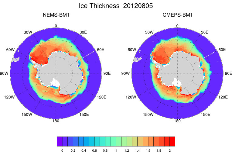
The comparison of the simulated sea ice concentration (Fig. 1a and 1b), thickness (Fig. 1c and 1d) and total ice area (Fig. 1e) for the NEMS-BM1 and CMEPS-BM1 simulations indicates that CMEPS-BM1 is able to reproduce the main characteristics and spatial distribution of the sea ice coverage as well as their evolution in time. Ice thickness analysis also shows that CMEPS-BM1 slightly underestimates the sea ice thickness in summer season especially in the area between 150E and 180E when compared to the baseline run (NEMS-BM1).
 |
| Figure 1.a: Comparison of spatial distribution of ice concentration (aice) in the Northern Hemisphere on the last day of the simulation (2012-02-05) for the run with January 2012 initial conditions. |
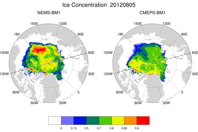 |
| Figure 1.b: Comparison of spatial distribution of ice concentration (aice) in the Northern Hemisphere on the last day of the simulation (2012-08-05) for the run with Jul 2012 initial conditions. |
 |
| Figure 1.c: Comparison of spatial distribution of ice thickness (hi, meter) in the Northern Hemisphere on the last day of the simulation (2012-02-05) for the run with January 2012 initial conditions. |
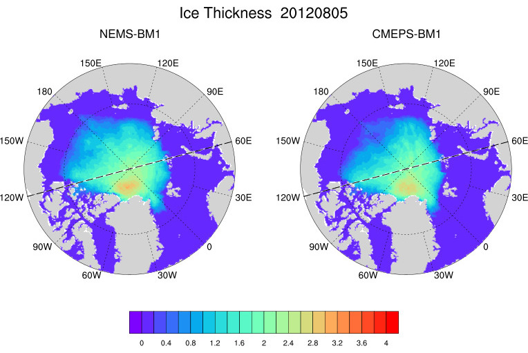 |
| Figure 1.d: Comparison of spatial distribution of ice thickness (hi, meter) in the Northern Hemisphere on the last day of the simulation (2012-08-05) for the run with July 2012 initial conditions. |
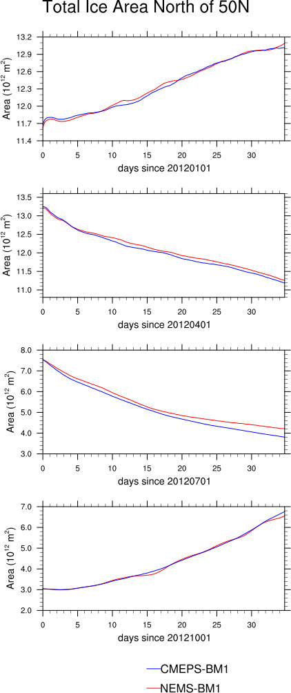 |
| Figure 1.e: Comparison of total ice area time series in the Northern Hemisphere for all seasons. |
A similar analysis is also available for the Southern Hemisphere. Plots for sea ice concentration (Fig. 2a and 2b), thickness (Fig. 2c and 2d), and total ice area (Fig. 2e) are included below. The analysis of ice concentration reveals that the CMEPS-BM1 simulation tends to have a positive bias in the winter season. This is also consistent with the ice area time series (Fig. 2e) and with the positive bias between NEMS-BM1 and CMEPS-BM1 starting to increase in time and reaching up to 1.0x10¹²m2 in the winter and spring seasons.
 |
| Figure 2.a: Comparison of spatial distribution of ice concentration (aice) in the Southern Hemisphere on last day of the simulation (2012-02-05) for the run with January 2012 initial conditions. |
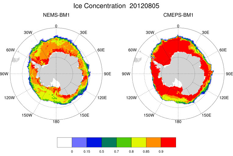 |
| Figure 2.b: Comparison of spatial distribution of ice concentration (aice) in the Southern Hemisphere on last day of the simulation (2012-08-05) for the run with July 2012 initial conditions. |
 |
| Figure 2.c: Comparison of spatial distribution of ice thickness (hi, meter) in the Southern Hemisphere on last day of the simulation (2012-02-05) for the run with January 2012 initial conditions. |
 |
| Figure 2.d: Comparison of spatial distribution of ice thickness (hi, meter) in the Southern Hemisphere on last day of the simulation (2012-08-05) for the run with July 2012 initial conditions. |
 |
| Figure 2.e: Comparison of total ice area time series in Southern Hemisphere for all seasons. |
As a part of initial validation analysis of CMEPS-BM1 simulations, the spatial distribution of the SST field and its anomaly from NEMS-BM1 simulation is also performed. For better evolution of the SST field, an animation of 6-hourly SST and anomaly maps is created from the results of the simulations for January and July 2012 periods (Fig 3a and 3b). As it can be seen from the figures, CMEPS-BM1 simulations are consistent with NEMS-BM1 and there is no spatial systematic bias between the simulations. In general the bias between model simulations are less than 0.5 oC but it increases slightly with time and becomes more evident.
 |
| Figure 3a: Animation of SST for January 2012 initial condition. |
 |
| Figure 3b: Animation of SST for July 2012 initial condition. |
In addition to the spatial analysis of SST field, the time-series for predefined regions are also calculated for further analysis of SST field and its evolution in time. Figure 4 shows the defined sub-regions.
 |
| Figure 4: Defined sub-regions that are used in the time-series analysis. |
Figures 5a and 5b show the evolution of SST for each defined sub-region (Figure 4). The results of CMEPS-BM1 simulations are very consistent with the results of NEMS-B1 simulations along with strong correlation (>0.8) and small RMSE error (0.02-0.59 oC) values (see Table 1). Unlike the winter and fall seasons, in which CMEPS-BM1 has better agreement with NEMS-B1, the CMEPS-BM1 simulation has positive bias in spring and summer seasons, which is more evident after day 15 of the simulations. This might be related with the difference of the surface heat flux components and accumulation of the error over the time, but further investigation is needed.
 |
| Figure 5a: SST time-series for January 2012 initial conditions. |
 |
| Figure 5b: SST time-series for July 2012 initial conditions. |
Table 1: The calculated Correlation Coefficients (CC) and Root-Mean-Square-Error (RMSE) values for SST between NEMS-BM1 and CMEPS-BM1 simulations.
| Jan | Apr | Jul | Oct | |||||
|---|---|---|---|---|---|---|---|---|
| CC | RMSE | CC | RMSE | CC | RMSE | CC | RMSE | |
| NINO 1+2 | 0.96 | 0.17 | 0.99 | 0.16 | 0.58 | 0.29 | 0.97 | 0.11 |
| NINO 3 | 0.94 | 0.13 | 0.64 | 0.59 | 0.96 | 0.11 | 0.87 | 0.07 |
| NINO 3.4 | 0.88 | 0.07 | 0.92 | 0.19 | 0.94 | 0.08 | 0.78 | 0.10 |
| NINO 4 | 0.68 | 0.10 | 0.97 | 0.09 | 0.61 | 0.10 | 0.81 | 0.18 |
| SATL | 0.98 | 0.07 | 1.00 | 0.08 | 0.96 | 0.08 | 0.93 | 0.13 |
| NATL | 1.00 | 0.02 | 0.92 | 0.15 | 0.99 | 0.08 | 1.00 | 0.06 |
| INDO | 0.82 | 0.14 | 0.94 | 0.20 | 0.89 | 0.10 | 0.81 | 0.18 |
The initial analysis of the surface heat flux components (shortwave and longwave radiation, latent and sensible heat fluxes) is summarized in Figures 6a and 6b. The results indicate a large systematic negative bias at the beginning of the CMEPS-BM1 simulation (2012-01-01_06:00:00 or 2012-07-01_06:00:00). This could be caused by a synchronization issue among the model components in the initialization phase, causing a small shift in model time. This needs to be investigated carefully by increasing the temporal resolution of output at the beginning of the simulation. There are also inconsistencies in the simulated net shortwave radiation between NEMS-BM1 and CMEPS-BM1. The error grows with time and starts to dominate the solution, which might also lead to differences in other flux components. The calculation of the net shortwave radiation by accounting its components (each individual band) in the Mediator should be reviewed to ensure correctness. Penetration of shortwave radiation under sea ice conditions should also be reviewed.
 |
| Figure 6a: Animation of surface heat flux components for January 2012 initial condition. Only 06h and 18h is used to create animation due to the file size restriction on GitHub. |
 |
| Figure 6b: Animation of surface heat flux components for July 2012 initial condition. Only 06h and 18h is used to create animation due to the file size restriction on GitHub. |