Seaborn is a library for making statistical graphics in Python. It is built on top of matplotlib and closely integrated with pandas data structures. — Seaborn website
- https://seaborn.pydata.org/
- https://github.com/mwaskom/seaborn
- https://seaborn.pydata.org/tutorial.html
- https://seaborn.pydata.org/examples/index.html
- https://www.datacamp.com/community/tutorials/seaborn-python-tutorial
- Styles: https://seaborn.pydata.org/generated/seaborn.set.html
Seaborn is designed to be more user-friendly and to work better with pandas dataframes. For more information on dataframes and the pandas package see here. It is also easier to customize plot colors, formats, etc. with Seaborn. Because seaborn is built on top of matplotlib, you will have to use commands from both packages for many operations.
Before diving into seaborn, make sure you brush up on your matplotlib skills! Click here for more information on matplotlib.
First install the package using Pip, if necessary:
pip install seabornConstructing a Scatterplot:
# adapted from https://seaborn.pydata.org/tutorial/relational.html

import matplotlib.pyplot as plt
import seaborn as sns

# The .set() function changes the plot's aesthetics
# For more information and specific styles see: https://seaborn.pydata.org/generated/seaborn.set.html
sns.set(style="darkgrid")

# The .load_dataset() function uses a built-in dataset
tips = sns.load_dataset("tips") # this is a pandas DataFrame!
print(type(tips)) #> <class 'pandas.core.frame.DataFrame'>
print(tips.columns.tolist()) #> ['total_bill', 'tip', 'sex', 'smoker', 'day', 'time', 'size']

# The .relplot() function creates a relational plot using an x-axis and y-axis
# It also allows you to specify the markers, colors, sizes, etc.
sns.relplot(x="total_bill", y="tip", hue="smoker", data=tips)

# Need to explicitly "show" the chart window
plt.show()
NOTE: once you "show" the chart, you'll see the chart open in native window on your computer. You'll be able to view your chart, but when you're done you'll need to close the chart window in order to regain the ability to type commands in your terminal window.
Consult the documentation and examples for a variety of chart customization options.
Reference: https://seaborn.pydata.org/_images/pairplot_1_0.png
sns.pairplot(df)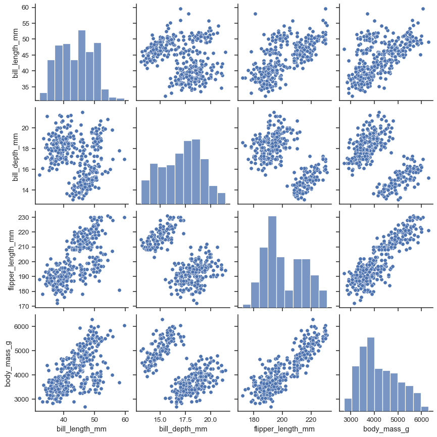
Reference: https://seaborn.pydata.org/generated/seaborn.heatmap.html
import matplotlib.pyplot as plt
import seaborn as sns

def plot_correlation_matrix(df, features):
    # https://pandas.pydata.org/pandas-docs/stable/reference/api/pandas.DataFrame.corr.html
    mat = df[features].corr(method="spearman")
    print(type(mat))

    sns.set(rc = {'figure.figsize':(10,10)})
    sns.heatmap(mat.T,
                square=True, annot=True, cbar=True,
                xticklabels=features,
                yticklabels=features,
                #vmin=0, vmax=1 # orient the color scale properly?

                # https://stackoverflow.com/questions/47461506/how-to-invert-color-of-seaborn-heatmap-colorbar
                cmap= "Blues" #"viridis_r" #"rocket_r" # r for reverse
    )
    plt.xlabel("Feature Name")
    plt.ylabel("Feature Name")
    plt.title("Spearman Correlation between features")
    plt.show()

plot_correlation_matrix()
from sklearn.metrics import confusion_matrix
import seaborn as sns
import matplotlib.pyplot as plt

def plot_confusion_matrix(clf, y_test, y_pred):
    """Params clf : an sklearn classifier """

    classes = clf.classes_

    cm = confusion_matrix(y_test, y_pred)
    # Confusion matrix whose i-th row and j-th column entry indicates the number of samples with
    # ... true label being i-th class and predicted label being j-th class.

    # df = DataFrame(cm, columns=classes, index=classes)

    sns.set(rc = {'figure.figsize':(10,10)})

    sns.heatmap(cm,
                square=True, annot=True, fmt="d", # format d shows integer values
                xticklabels=classes,
                yticklabels=classes,
                cbar=True, cmap= "Blues" #"Blues" #"viridis_r" #"rocket_r" # r for reverse
    )

    plt.ylabel("True Genre") # cm rows are true
    plt.xlabel("Predicted Genre") # cm cols are preds
    plt.title("Confusion Matrix on Test Data (Logistic Regression)")
    plt.show()


plot_confusion_matrix(my_classifier, y_test, y_pred)