Dynamic Programming (DP) is a similar approach to Divide & Conquer. It also breaks the problem into similar subproblems, but they are actually overlapping and codependent — they’re not solved independently. Each subproblem’s result can be used anytime later and it is built using memoization (precalculation). DP is mostly used for (time & space) optimization and it is based on finding a recurrence.
A method which describes algorithm complexity, the execution time required or the space used in memory by an algorithm, where "n" represents size of the data structure.
Describe the rough estimate of the number of "steps" to complete the algorithm.
- Rules:
- O(1) * O(n) = O(n) ------------ do something n times => loop
- O(n) * O(n) = O(n^2) ------------ outer loop runs n times * inner loop runs n times (nested loop)
- O(1) + O(n) = O(n) ------------ constant time + loop
- O(n) + O(n^2) = O(n^2) ---------- loop + loop with nested loop
- O(1) + O(n) + O(n^2) = O(n^2)
- O(1) + O(n/2) + O(100) = O(n) --- As n gets really big, any operation has a decreasingly significant effect
- O(n^3 + 50n^2 + 10000) = O(n^3)
- O((n+30) * (n+5)) = O(n^2)
Assuming "n" becomes very large, the notation with slower increase speed could be ignored 🐌 (as the nature of large scale data in computer engineering, everything else is quickly eclipsed as n gets very large)
-
Speed:
O(1) < O(log(n)) < O(n) < O(n log(n)) < O(n^2) -
Sort Algorithms (Worst case):
- Mergesort, Timsort, Heapsort =
O(n log(n)) - Quicksort, Bubble Sort, Insertion Sort, Selection Sort =
O(n^2)
- Mergesort, Timsort, Heapsort =
About memory cost, to optimize an algorithm for using less memory.
When comparing different algorithms, we often compare how much "extra" space complexity is needed to solve the problem.
In an algorithm, we need to create an array of size n to store the temporary results before getting the final result. If we assume that the size of a element in the array is a constant "C" which is independent to "n", the space complexity for using the array is Cn which is O(n) * O(C) = O(n) * O(1) = O(n)
O(1) space complexity if more efficient than O(n)
- Data Structures:
- Array, Stack, Queue, Hash Table, BST =
O(n) - Skip list =
O(n log(n))
- Array, Stack, Queue, Hash Table, BST =
- Sort Algorithms:
- Heapsort, Bubble Sort, Insertion Sort, Selection Sort =
O(1) - Quicksort =
O(log(n)) - Mergesort, Timsort =
O(n)
- Heapsort, Bubble Sort, Insertion Sort, Selection Sort =
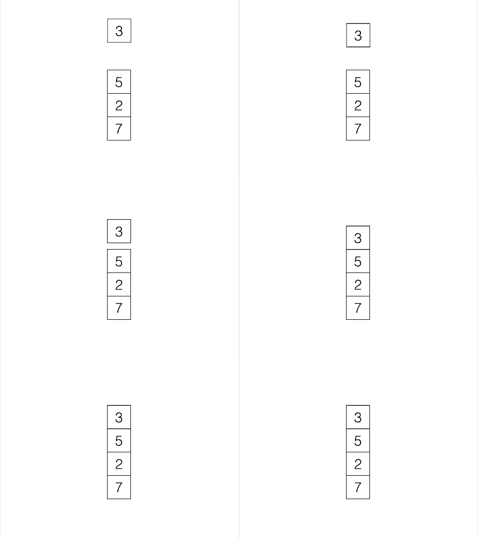
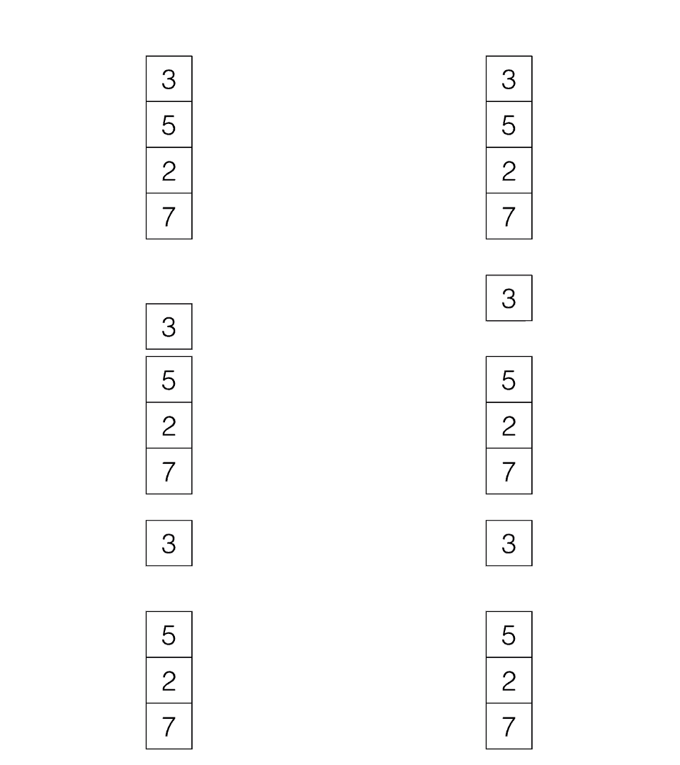
Last In, First Out, e.g: Stacks
 |
 |
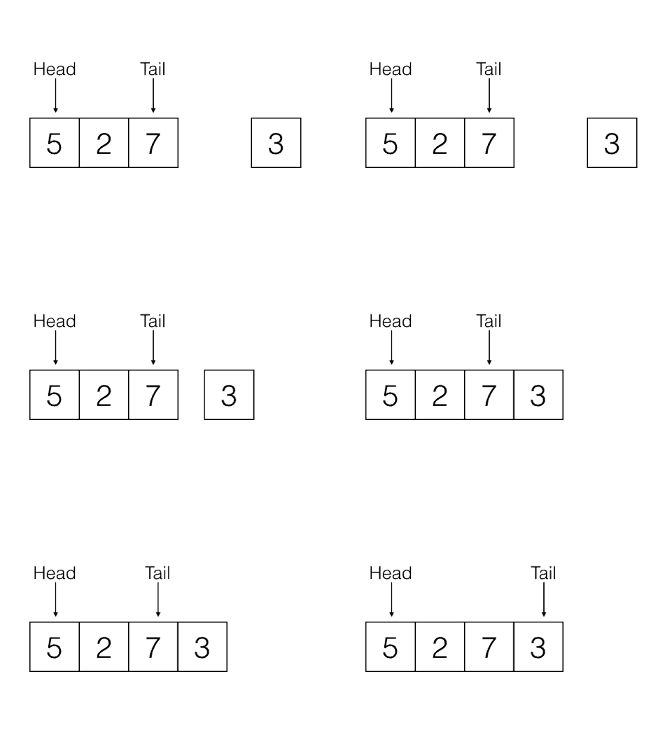
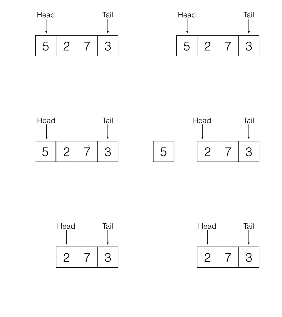
First In, First Out, e.g: Queues
 |
 |
A stack data structure that stores information about the active subroutines of a computer program. (also known as an execution stack, program stack, control stack, run-time stack, or machine stack). It's used to keep track of the point to which each active subroutine should return control when it finishes executing. An active subroutine is one that has been called, but is yet to complete execution, after which control should be handed back to the point of call.
Graphs are used to represent networks. It's a data structure that consists of the following two components:
- A finite set of vertices also called as nodes.
- A finite set of ordered pair of the form (u, v) called as edge. The pair of the form (u, v) indicates that there is an edge from vertex u to vertex v. The edges may contain weight/value/cost. Example:
  (u, v)
[0] -- [1]
 |    /   \
 |   /     [2]
 |  /     /
[4] -- [3]A 2D array of size V x V where V is the number of vertices in a graph (used to represent weighted graphs). e.g:
[[0, 1, 0, 0, 1],
 [1, 0, 1, 0, 1],
 [0, 1, 0, 1, 0],
 [0, 0, 1, 0, 1],
[1, 1, 0, 1, 0]];- Consumes more space O(V^2).
- Adding a new vertex the storage must be increases to (|V|+1)^2, complexity is O(V^2).
- Adding an edge requires O(1) time.
- Removing a vertex the storage must be decreased to V^2 from (|V|+1)^2, complexity is O(V^2).
- Removing an edge takes O(1) time.
- Finding for an existing edge, given two vertices, can be checked in O(1) time.
A graph is represented as an array of linked list. The size of the array is equal to the number of vertices.
[
  [1, 4],
  [0, 2, 4],
  [1, 3],
  [2, 4],
  [0, 1, 3]
];- Saves space O(|V|+|E|).
- Adding a vertex is easier O(1).
- Adding an edge requires O(1) time.
- Removing a vertex takes O(|V|+|E|) time (search for the vertex and traverse the edges).
- Removing an edge takes O(|E|) time (traversing through the edges).
- Queries like whether there is an edge from vertex u to vertex v are not efficient and can be done O(V).
Refers to the process of visiting (checking and/or updating) each node in a tree data structure, exactly once. As a tree is a self-referential (recursively defined) data structure, traversal can be defined by recursion or, more subtly, corecursion, in a very natural and clear fashion; in these cases the deferred nodes are stored implicitly in the call stack.
Involves iterating over all nodes in some manner:
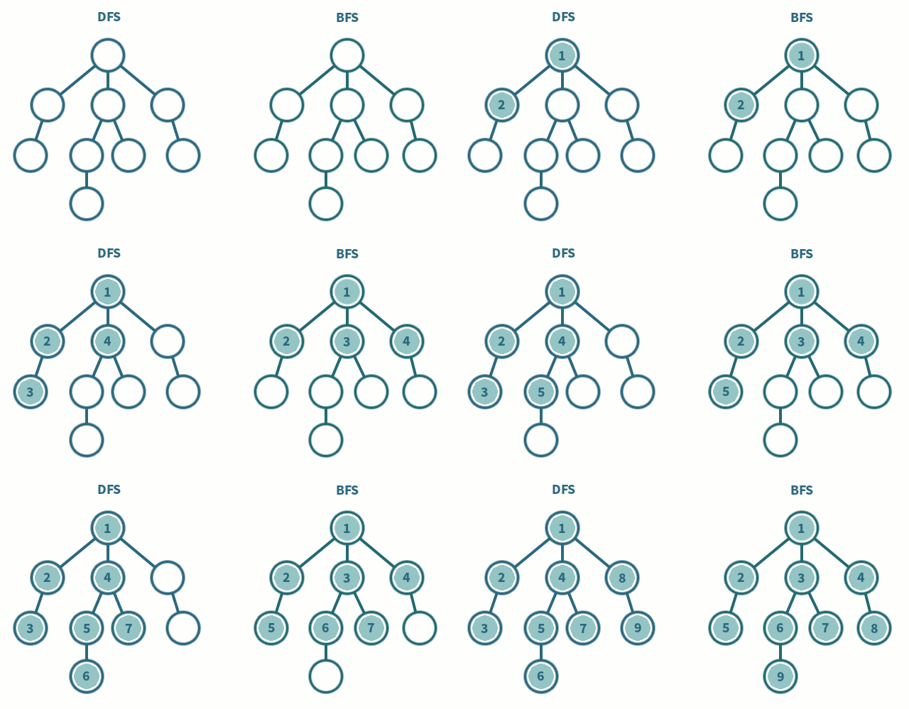
Starts at the root node and explores as far as possible along each branch before backtracking, with a DFS you push the children of the current node onto a stack, so they will be popped and processed before everything else. It's easily implemented via a stack, including recursively via the call stack:
- Pre-order (NLR): It's a topologically sorted one, because a parent node is processed before any of its child nodes is done.
- In-order (LNR): Retrieves the keys in ascending sorted order.
- Reverse in-order (RNL): Retrieves the keys in descending sorted order.
- Post-order (LRN): The trace of a traversal is called a sequentialisation of the tree. The traversal trace is a list of each visited root.
Starts at the tree root and explores all of the neighbor nodes at the present depth prior to moving on to the nodes at the next depth level, with a BFS you push the children onto the end of a queue, so they will be popped and processed after everything else. It's easily implemented via a queue, including corecursively.
- Tech Interview Handbook
- Coding Interview University
- Complete Introduction to the 30 Most Essential Data Structures & Algorithms
- Introduction to Big O Notation and Time Complexity
- To study runtime complexity: Big O Cheat Sheet
- The ultimate guide for data structures & algorithm interviews
- OOP Principles For Dummies
- Graph Algorithms
- Queues and Stacks
